Welcome to Geodata’s documentation!#
Geodata is a Python library of geospatial data collection and analytical tools. Through the creation of shared scripts and documentation for analysis-ready physical variables, geodata streamlines the collection and use of geospatial datasets for natural science, engineering, and social science applications.
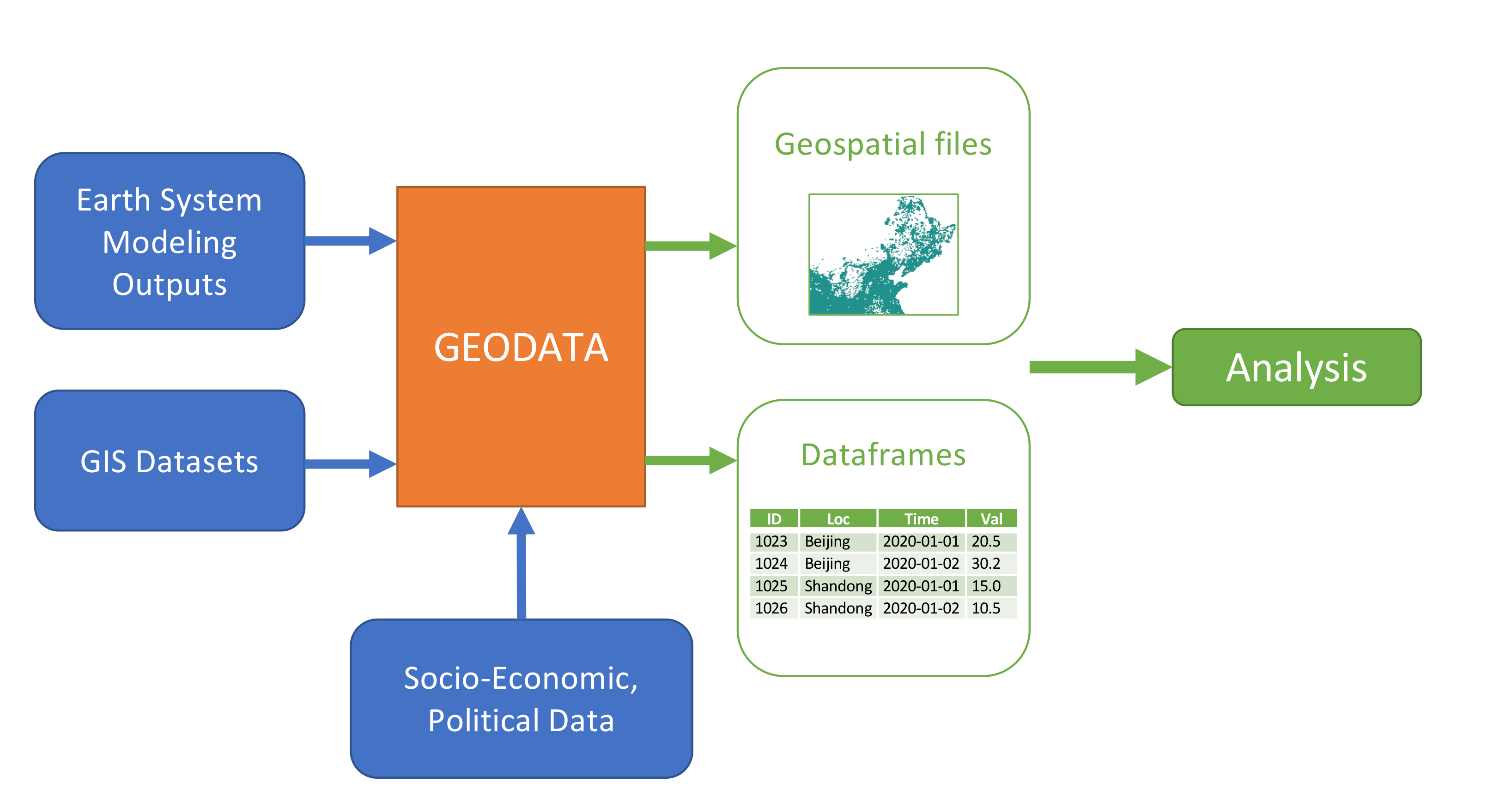
A typical analysis workflow with Geodata#
Motivation#
The main motivation is the difficulty in working with high temporal and spatial resolution datasets of physical variables from earth system models and combining them with GIS datasets (land use, geographic features, etc.). The primary analytical questions addressed here are generating profiles of energy and environmental variables of interest (solar PV, wind power, pollution distribution) subject to suitability and weighting criteria. Additional applications are under development.
Working with these datasets has startup costs and computational barriers due to diverse sources, formats, resolutions, and large memory requirements. To solve this, geodata provides an all-in-one Python interface for downloading, subsetting, and transforming large earth systems datasets into relevant physical variables and flexibly incorporating GIS datasets to mask these variables and generate “analysis-ready” datasets for use in regression, plotting, and energy models. Geodata builds off the structure of the atlite package.
How To Use#
Installation#
In short, Geodata is available on PyPI and can be installed via pip:
pip install geodata-re
For more detailed installation instructions, see the installation guide.
Download Datasets#
Earth system datasets can be large (100+ MB / file with hundreds of files necessary for a single analysis) and their APIs and file structures (e.g., daily vs monthly) vary by source. Utilizing xarray and dask data parallelization, geodata provides single call download with API credentials stored locally. Data requests are automatically trimmed to keep only required variables, significantly reducing bandwidth requirements and disk usage.
Geodata currently supports MERRA-2 and ERA5 reanalysis products and various GIS file formats (see here). For example, to evaluate solar PV availability using MERRA2 on 01/01/2011, use the following method call:
from geodata import Dataset

solar = Dataset(
   module="merra2",
   years= slice(2011, 2011),
   months=slice(1,1),
   weather_data_config="slv_radiation_hourly"
)
solar.get_data()
Extract Cutouts [ADD edit this section]#
Most energy analyses (e.g., energy models, resource assessments,
political economy studies) require time series on subsets of locations
and time periods. Geodata can extract desired variables, time periods,
and geographies from the dataset to a Cutout object. We then call various
conversion methods of the Cutout class to transform the raw data
into analysis-ready variables with the option to export to CSV or combine with other
GIS datasets through further masking analysis.
After downloading the required MERRA2 dataset, we create a Cutout object that contains solar irradiance over China.
from geodata import Cutout

cutout = Cutout(
   name="china-2011-slv-hourly-test",
   module="merra2",
   weather_data_config="slv_radiation_hourly",
   xs=slice(73, 136),
   ys=slice(18, 54),
   years=slice(2011, 2011),
   months=slice(1, 1),
)
cutout.prepare()
Then, we can convert the downward-shortwave, upward-shortwave radiation
flux, and ambient temperature variables from the Cutout data into a PV
generation time-series using the cutout’s pv method. Geodata
stores objects internally as an xarray DataArray, which can be easily
converted to a Pandas DataFrame.
ds_solar = cutout.pv(panel="KANEKA", orientation="latitude_optimal")
ds_solar.to_dataframe(name="pv")
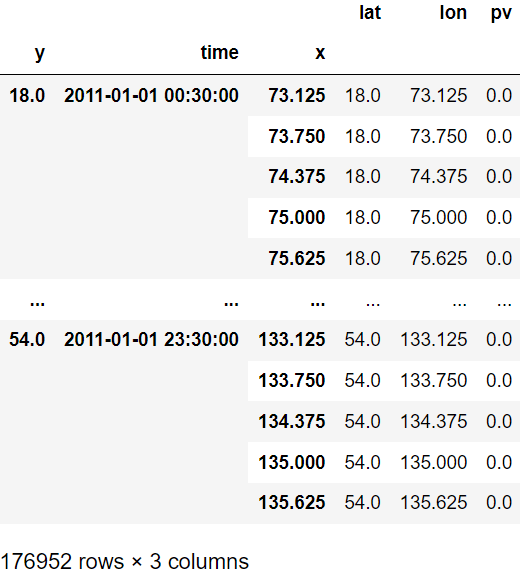
Output of the code above#
We can plot a time series of average PV values for all grid cells on that day with geodata’s visualization method:
from geodata import plot

plot.time_series(ds_solar)
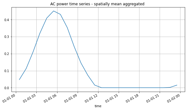
Visualization of the average PV values over time#
We can also visualize the average solar PV for every two hours on this day through an animation:
import geopandas as gpdø

from geodata import plot

prov_shapes = gpd.read_file(prov_shapes_path)
geodata.plot.heatmap_animation(
   ds_solar,
   cmap="Wistia",
   time_factor=2,
   shape=prov_shapes,
   shape_width=0.25,
   shape_color="navy",
)
Animated Result#
Wind Speed Modeling#
Estimating wind speed and wind generation from simulated reanalysis or weather models entails a number of assumptions, due to the general sparsity of measurements and complex meteorology affecting wind speed evolution with height.
The model module extracts multiple wind speeds from the underlying datasets which are used to support wind speed estimation in one of two ways: interpolation and extrapolation.
from geodata import Cutout
from geodata.model.wind import WindExtrapolationModel

cutout = Cutout(
   name="china-2011-slv-hourly-test",
   module="merra2",
   weather_data_config="slv_flux_hourly",
   xs=slice(73, 136),
   ys=slice(18, 54),
   years=slice(2011, 2011),
   months=slice(1, 1),
)
cutout.prepare()

model = WindExtrapolationModel(cutout)
model.prepare()

windspd = model.estimate(height=100, years=slice(2011, 2011), months=slice(1, 1))
windspd.to_dataframe(name="wind")
Masking#
Geographic masks help filter datasets for specific analyses. Geodata is able to process GIS datasets and extract cutouts over specified geographies. Built off the open-source binary libraries GDAL, GEOS, and PROJ, and Python libraries rasterio and shapely, the Mask module imports rasters and shapefiles, edits them as mask layers, merges and flattens multiple layers together, and extracts subsetted cutout data from merged masks and shapefiles.
For example, within Geodata the user can load the MODIS land use dataset, the elevation dataset, and environmental protected shapes, filter these according to solar energy suitability criteria, and merge into a single binary siting mask, where values of 0 represent the unsuitable area, and values of 1 represent the suitable area. Masks can be saved locally for later use.
Geodata automatically reprojects GIS data in different coordinate
reference systems into degree coordinates for processing. Common
manipulations include cropping, filtering on categorical values,
filtering on thresholds, excluding small contiguous areas, and filtering
by shape buffers. One multi-purpose plotting function (mask.show)
supports visualizing the mask including relevant shape boundaries.
For example, Geodata can create a binary mask of wind energy suitability in China based on the above GIS inputs.
import geopandas as gpd

from geodata import mask

china = mask.Mask("China")
china.add_layer(layer_path={"modis": modis_path, "elevation": elevation_path})

protected_area_shapes = gpd.read_file(protected_area_shapes_path)
china.add_shape_layer(
   protected_area_shapes["geometry"].to_dict(),
   reference_layer="elevation",
   combine_name="protected",
   buffer=20,
)

china.filter_layer(
   "modis", binarize=True, values=[6, 7, 8, 9, 10, 11, 12, 14, 15, 16, 17]
)
china.filter_layer("elevation", binarize=True, max_bound=4000)
china.merge_layer(trim=True)

china_prov_shapes = gpd.read_file(china_prov_shapes_path)
mask.show(china.merged_mask, shape=china_prov_shapes["geometry"], title="Merged Mask")

china.save_mask()
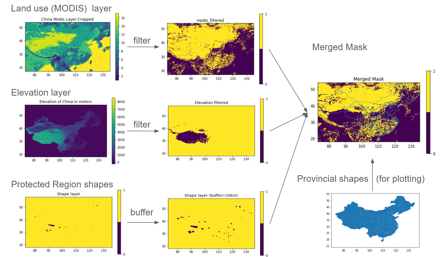
Visualization of Mask Workflow#
In the final step, we apply the Mask object to the Cutout. Geodata automatically coarsens the (typically) high-resolution Mask into the same resolution as the Cutout, adding fractions of the coarse cells covered by the Mask and areas calculated via an equal-area projection.
ds_cutout = cutout.pv(
   panel="KANEKA", orientation="latitude_optimal"
).to_dataset(name="solar")

cutout.add_mask("china")
cutout.add_grid_area()
ds_mask = cutout.mask(dataset=ds_cutout)["merged_mask"]

weighted_mean_pv_series = (
   (ds_mask["solar"] * ds_mask["mask"] * ds_mask["area"]).sum(axis=1).sum(axis=1)
) / (ds_mask["mask"] * ds_mask["area"]).sum()

plt.plot(weighted_mean_pv_series)
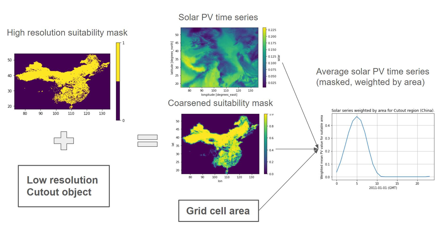
Mask-Cutout Workflow#
What’s next?#
To further explore the capabilities of Geodata, check out the table of contents on the left!